Determination of Cd by Differential Pulse Voltammetry by using TFME
Introduction
Differential pulse voltammetry (DPV) is a technique that involves applying amplitude potential pulses on a linear ramp potential. In DPV, a base potential value is chosen at which there is no faradaic reaction and is applied to the electrode.
The major advantage of DPV is low capacitive current, which leads to high sensitivity. The small step sizes in DPV also lead to narrower voltammetric peaks and thus DPV is often used to discriminate analytes that have similar oxidation potentials.
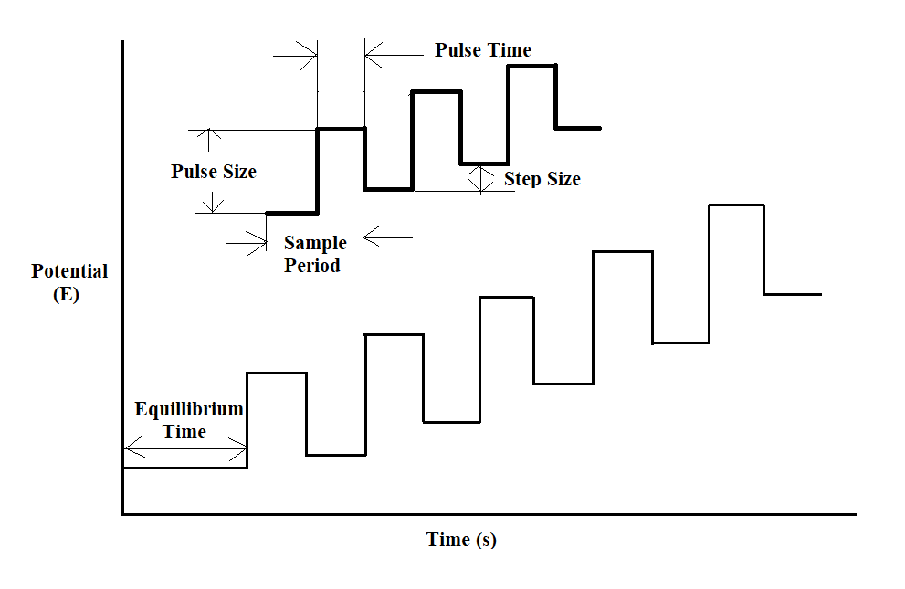
Figure 1: Potential wave form for differential pulse voltammetry
The potential wave form consists of small pulses (of constant amplitude) superimposed upon a staircase wave form. Here, the current is sampled twice in each Pulse Period (once before the pulse, and at the end of the pulse), and the difference between these two current values is recorded and displayed.
Differential pulse voltammetry (DPV) is important for the determination of pharmaceuticals, dyes, insecticides and pesticides.
Experimental Part
Instrumentation
In this experiment a compact and portable potentiostat, PhadkeSTATTM20 which runs on “EC-Prayog” a Windows based software was used.
Requirements
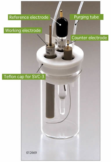
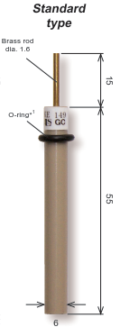
A three electrode voltammetry cell for the electrochemical reaction to take place. Three electrode were used; a Glassy carbon working electrode electrode, a Ag/AgCl reference electrode, a Platinum counter electrode. The working electrode was cleaned by lightly polishing with alumina and then was rinsed with water. A micropipette (range from 100ul-1000ul) The connection between potentiostat and the cells were: Green= working; White= reference; Red= counter; Black= ground.
(a)
(b)
(c)
(d)
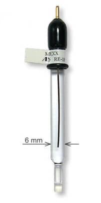
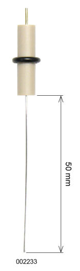
Figure 2: From left to right (a) SVC-3 Voltammetry Cell (b) Reference electrode (Ag/AgCl) (c) Counter electrode (Pt Wire) (d) Working electrode (Glassy Carbon)
Reagent
All solutions should be prepared fresh and All the glassware should be soaked, preferably overnight in 3 M HN03 and rinsed several times with deionised water.
Acetic acid (CH3COOH), ammonia (NH3), Cadmium sulphate (3CdSO4.8H2O), Hg standard stock solution (1000ppm), Hydrochloric acid (HCl) and Distilled Water.
Preparation of Standard solution (Cd Standard)
To prepare 1000ppm of Cd standard, weigh out 0.228g of 3CdSo4.8H2O and dissolve in distilled water in a 100ml Standard flask then make it up to the volume and mix well. Then prepare a solution of concentration 100ppm by serial dilution method.
Preparation of supporting electrolyte
(Ammonium acetate buffer)
11.1 ml of acetic acid was taken in a 100ml volumetric flask, to this 20 ml of distilled water was added. 7.4ml of ammonia was slowly added to the volumetric flask. Ammonia has to be added slowly, because of the generation of heat while addition. After the addition of ammonia, the solution was diluted to 100ml with distilled water. The pH of the buffer is 4.6.
Preparation of Hg plating solution
Take a 20 ml standard flask, Pipette out 0.4ml of mercury standard stock solution and then add 0.2ml hydrochloric acid to the flask then dilute the volumetric flask up to the mark with distilled water. This solution can be reused several times and should be stable for a month.
Nitrogen Gas
Used for purging to remove oxygen.
Procedure
Preparation of thin film mercury electrode
Preparation of Glassy Carbon electrode for mercury film plating:
Clean the GC electrode with soft tissue, then the electrode is polished with electrode polishing kit; it is explained in detail in this article. The electrode is then rinsed with acetone and afterwards thoroughly with distilled water.
Plating of mercury film on GC electrode:
Here TFME is prepared in situ by adding the mercury plating solution directly into the supporting electrolyte and analyte at -0.4V for 300 seconds. TFME can be prepared separately by plating mercury in a different solution then used in analyte. Once the TFME is generated, it must be protected from oxygen to prevent oxidation of the film.
Take 8ml of supporting electrolyte in the SVC-3 cell and add 2ml of the mercury plating solution and then connect the electrodes as explained earlier. (make sure electrodes are dipped in the solution). Turn on N2 gas cylinder start the purging process for 30-45 minutes.
After the purging is complete, open the PhadkeSTATTM20 software ‘EC-Prayog’ and switch on the potentiostat. Connect the potentiostat to the computer for the software to communicate with the potentiostat
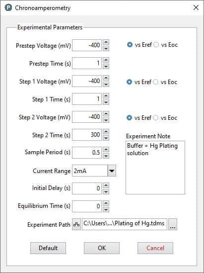
Go to Experiment menu and select Chronoamperometry
After selection of Chronoamperometry, the Experimental Parameters box will open. Set the parameters as suggested below, you may change the parameters appropriately as per your requirement.
Figure 3: Chronoamperometry (Plating of Mercury)
After TFME is prepared, sample is ready to be analysed.
In the same solution of Buffer and mercury plating solution in the voltammetry cell add 1ml of Cd standard solution (100ppm), making the resultant concentration of the solution (mixture of buffer, Hg plating solution and Cd standard) 9 ppm.
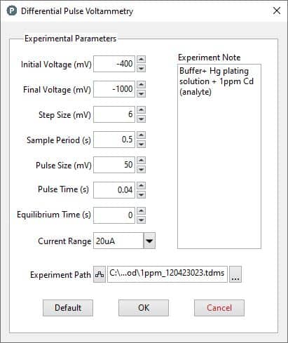
Go to Experiment menu to select Differential Pulse Voltammetry (DPV) technique.
After selection of Differential Pulse Voltammetry, the Experimental Parameters box will open. Set the parameters as suggested below, you may change the parameters appropriately as per your requirement.
Once the parameters have been set, the experiment can be started by clicking OK, in the Experiment menu.
Keep on increasing the concentration of the solution by adding 1ml and repeat the experiment for different concentration
Repeat the step “Plating of mercury” step 3-d before each experiment
After the experiment is concluded, go to the Analysis menu, a new tab will open showing the saved experiment files, select the file to be analysed another new tab will open; that is the Analysis window.
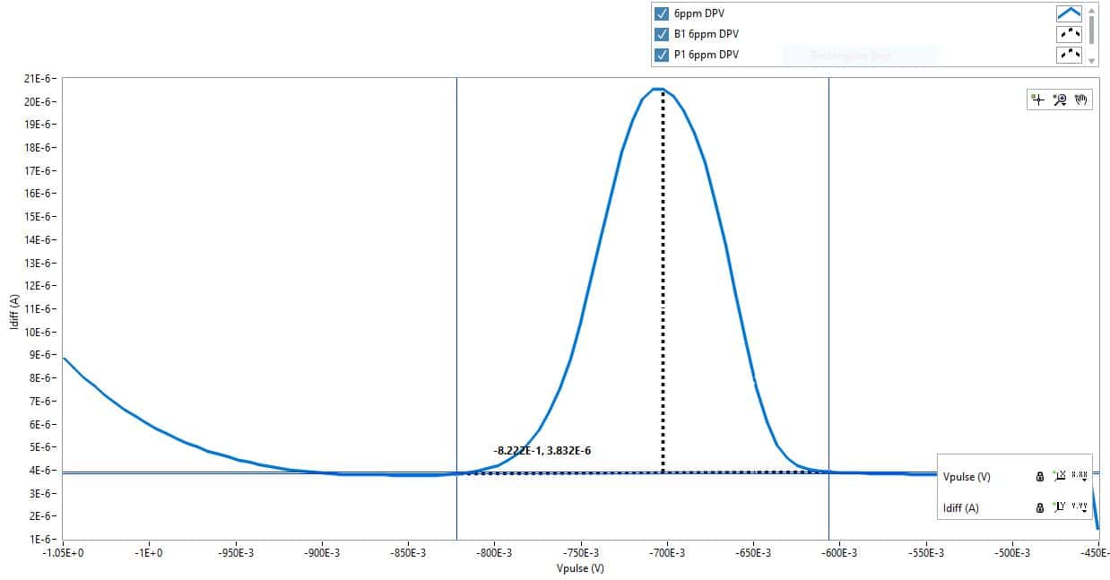
In the analysis window firstly select the file to be analysed, and then click on Start Analysis, then select both the cursor Cursor 1 and Cursor 2, to find the peak on the graph manually. Move the cursor to the one end of the “peak” of the voltammogram and select a linear portion. Do the same thing at the other end of the “peak” of the voltammogram and then select Draw Baseline & find Peak.
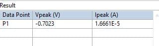
After getting the peak click on display result to get numerical values of these peak parameters.
Figure 6: DPV Results
Effect of concentration
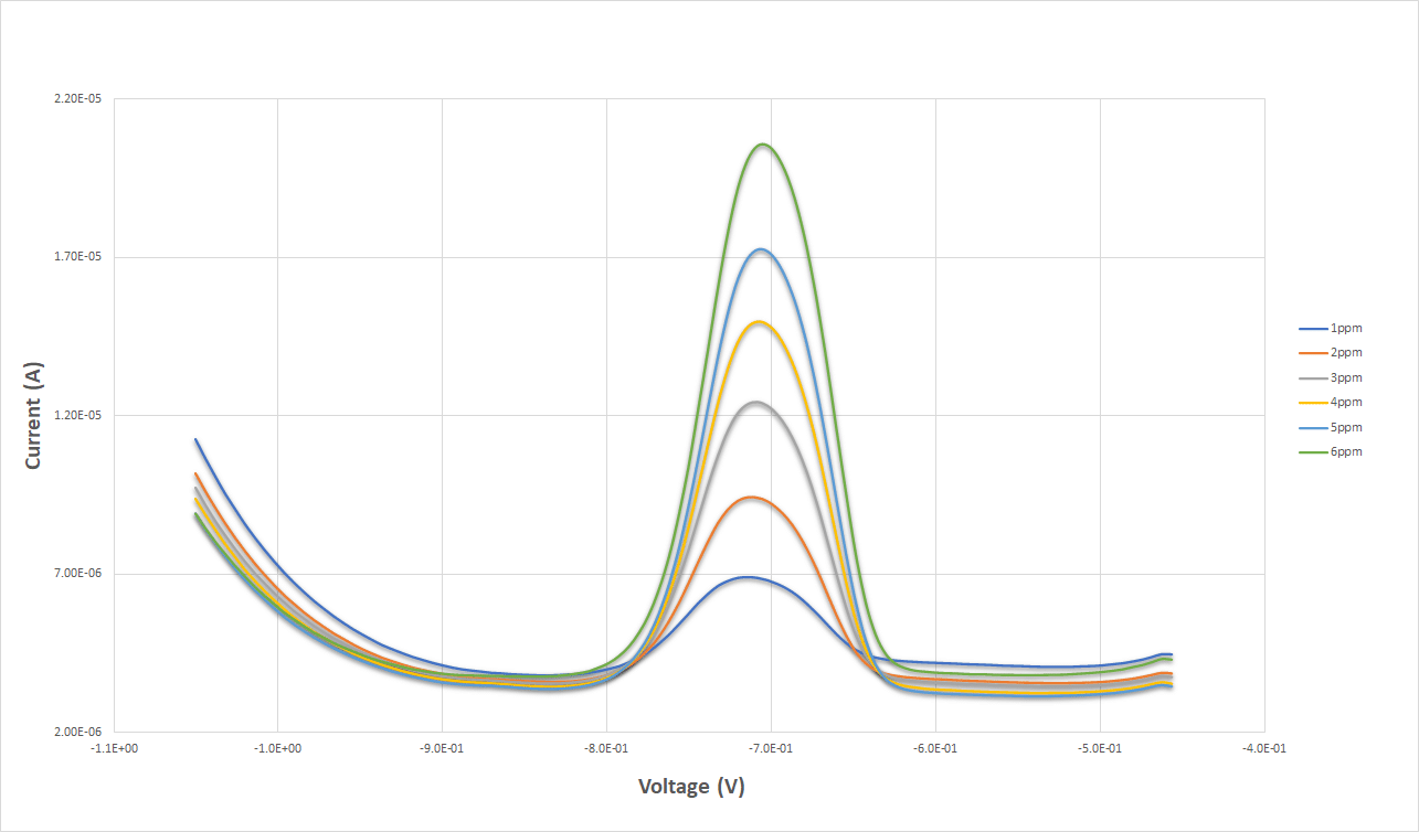
Overlay of the voltammogram for each concentration is displayed in following graph,
Figure 7: Overlay of Differential pulse voltammograms of Cadmium standard in Ammonia Acetate Buffer by TFME are illustrated below. Concentrations = 1, 2, 3, 4, 5 and 6ppm
Concentration dependence on the peak currents can be shown by plot of ip conc.
Figure 8: The peak current increases linearly with the concentration of the analyte.