This article describes an experiment for an undergraduate chemistry laboratory to introduce cyclic voltammetry prior to studies of more complex systems. It also serves as a general introduction to computer based instrumentation.
Introduction
Cyclic Voltammetry is an electrochemical technique for the study of electro-active species which measures the current that develops in an electrochemical cell under conditions where voltage is in excess of that predicted by the Nernst equation. It is widely used in industrial applications and academic research laboratories
Figure 1: Electrochemical redox conversion between ferricyanide and ferrocyanide.
In this article, the FeIII(CN)63-/FeII(CN)64- couple is used as an example of an electrochemically reversible redox system in order to introduce some of the basic concepts of cyclic voltammetry. The resulting voltammogram can be analysed for fundamental information regarding the redox reaction. The PhadkeSTAT 20 is ideal for performing electrochemical experiments. The instrument is simple to use, and its Windows-based software can be quickly mastered by students with little or no background in electrochemistry.
Experimental
Reagents
A 100mL stock solution of 5mM K3Fe(CN)6 in 0.1N KCl is prepared. Weigh 164 mg of K3Fe(CN)6 and put in the volumetric flask. Add 745 mg KCl and add about 50ml water. Swirl the flask till both the salts dissolve. Add 1 drop of dilute H2SO4 and dilute up to the mark.
Apparatus
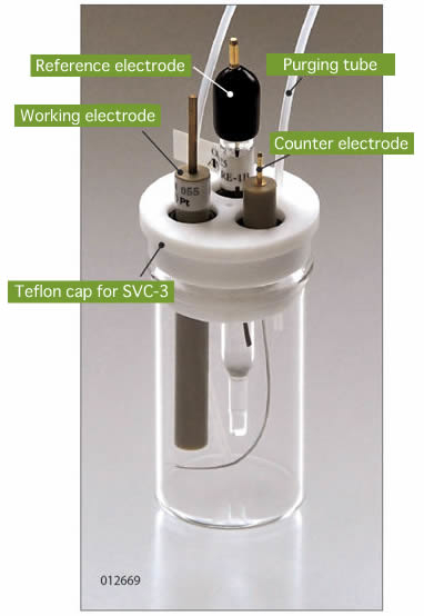
In this experiment a compact and portable potentiostat, PhadkeSTAT 20 which runs on “EC-Prayog” a Windows supporting software was used. (Note: The software has a Device status indicator where Grey = Not connected Blue = Device is connected Green = Device is running) A 3- electrode voltammetry cell for the electrochemical reaction to take place. Three electrodes were used; a Glassy carbon working electrode (ALS, Japan) (OD = 6mm; ID = 3mm), a silver/silver chloride reference electrode (RE-1B, ALS, Japan) (L = 78mm; D = 6mm) and a counter electrode (Length = 50mm). The working electrode was cleaned by lightly polishing with alumina and then was rinsed with water. Alternately a carbon screen printed electrode SPE can be used. The connection between potentiostat and the cells were: Green= working electrode; White= reference electrode; Red= counter electrode; Black= ground.
(a) SVC-3 Voltammetry Cell
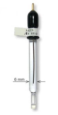
(b) Reference electrode (Ag/AgCl)
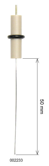
(c) Counter electrode (Pt Wire)
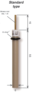
(d) Working electrode (Glassy Carbon)
Figure 2: From left to right (a) SVC-3 Voltammetry Cell (b) Reference electrode (Ag/AgCl) (c) Counter electrode (Pt Wire) (d) Working electrode (Glassy Carbon).
Procudure
A. Running CV
1.Add 5-10ml solution of 5mM K3Fe(CN)6 into the SVC-3 voltammetry cell (enough solution for the electrodes to be dipped in it) and then connect the electrodes as explained earlier. If an SPE is used, 1 drop of solution was put on the electrode so that all the 3 electrodes were covered with the solution.
2.Open the PhadkeSTAT 20 software ‘EC-Prayog’ and switch on the potentiostat. Connect the potentiostat for the software to communicate with the potentiostat.
3.Go to Experiment menu to select cyclic voltammetry (CV) technique.
4.After selection of cyclic voltammetry, the General Parameters box will be open. Enter the Experimental Parameters dialog box will open automatically, set the parameters as suggested below, you may change the parameters appropriately as shown in figure below.
Figure 3: Cyclic voltammetry parameter
After clicking on OK, the experiment is commenced and first OCP (Open Circuit-Potential) is measured as the equilibrium potential between the working and reference electrode when no net current flows within the circuit.
The graph of OCP is plotted as potential v/s time and ideally if the trend of the OCP graph gives a stable value it means the equilibrium has been reached.
Figure 4: Open Circuit Potential
6.After the OCP is completed, the voltammogram will appear on screen as it is generated and it will be rescaled automatically upon conclusion. Below is the CV of 5mM K3Fe(CN)6 in 0.1N KCl. (Note: We have selected total 2 cycles.)
After the experiment is concluded, go to the Analysis menu, a new tab will open showing the saved experiment files, select the file to be analysed another new tab will open; that is the Analysis window.
In the analysis window firstly select the cycle which you want to analyse and then click on Start Analysis, then select both the cursor Cursor 1 and Cursor 2, to find the peak on the graph manually. Select a linear portion with both the cursor at one end of oxidised wave then after that click on Anodic Baseline to create a baseline then move one cursor to the other end of the wave and there select a linear portion and then click on Anodic Peak for peak formation, repeat the same procedure for the analysis of reduced wave form.
Figure 7: Analysis of cyclic voltammogram
9.After getting both anodic and cathodic peak click on display result to get numerical values of these peak parameters.
B.The Effect of Scan Rate
Select Experimental Parameters from the main menu and change the scan rate from 10 mv/s to 20 mv/s. Run the experiment again and save the data. Repeat this procedure for scan rates of 40, 60, 80 and 100 mv/s.
The CVs for each scan rate can all be displayed on the same graph using Multi Graph in the Graphics menu. Cyclic voltammograms of 5mM K3Fe(CN)6 in 0.1N KCl are illustrated below. Scan rates = 10, 20, 40, 60, 80 and 100mV/s.
Figure 9: Overlay of Cyclic voltammograms of 5mM K3Fe(CN)6 in 0.1N KCl from Scan rates 10, 20, 40, 60, 80 and 100mV/s. At higher scan rates the rate of diffusion is more than the rate of reaction. Hence, more electrolytic ions reach the electrode electrolyte interface whereas very few ions participate in the charge transfer reaction. Therefore, the current at higher scan rate increase. Therefore, peak height increases with increase in scan rate. This is also evidenced by the increased voltage difference between anodic and cathodic peaks at higher scan rates.
3. The scan rate dependence of the peak currents and peak potentials can be shown two ways: by plot of ip vs. (scan rate)1/2,